The beauty of L-Systems

Vous pouvez aussi lire cet article en version française.

What are L-systems?

A Lindenmayer System (commonly referred to as L-system) is a recursive algorithmic model inspired by biology invented in 1968 by hungarian biologist Aristid Lindenmayer.

It aims to provide a way to model the growth of plants and bacterias.

The core concept behind L-systems is rewriting, an effective way to generate complex objects by replacing parts from a simple initial object.

We can see it as cell which divide at each iteration to generate a more complex organism.

If you feel curious, wikipedia offers a more complete description of it.

Ok, but why should you care about it, and most importantly, what can you achieve using it?

Well… a lot of things, even generating some music, but we’ll focus on visual applications, the illustrations on the banner of this post were generated using l-systems.

Imagine you want to break the monotony of a page, adding a crazy animated/generated/randomized pattern or you’re working on a game and want to add some deco or you’re simply interested in getting started with generative art, L-Systems will surely be a good start.

The structure of an L-system

First let review the structure of an L-system (the formal grammar), it’s comprised of:

• V a set of replaceable symbols (variables)
• S a set of non replaceable symbols (constants)
• ω a string of symbols from V defining the initial state of the system (axiom)
• P a set of production rules, defining how symbols from V should be replaced with constants (S) and/or variables (V)

An L-system is defined as a tuple and noted {V, S, ω, P} and sometimes {V, ω, P} (V and S being merged in V).

First take: the Koch curve

We’ll start with a variant of the Koch curve.

• variables V: F
• constants S: +, -
• axiom ω: F
• rules P: F → F+F-F-F+F

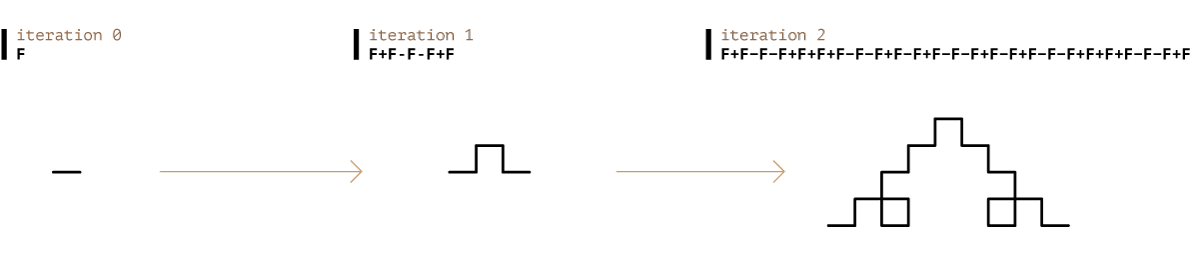
which will produces:

iteration 0 : F
iteration 1 : F+F-F-F+F
iteration 2 : F+F-F-F+F+F+F-F-F+F-F+F-F-F+F-F+F-F-F+F+F+F-F-F+F

The generation is quite easy to implement in javascript:

const lSystem = ({ axiom: ω, rules: P, iterations: N = 1 }) =>
[...Array(N).keys()]
.reduce(acc => acc.split('').map(s => P[s] ? P[s] : s).join(''), ω)

const result = lSystem({
axiom: 'F',
rules: { F: 'F+F-F-F+F' },
iterations: 2,
})

So, after 2 iterations, you should have this result:

  F+F-F-F+F+F+F-F-F+F-F+F-F-F+F-F+F-F-F+F+F+F-F-F+F

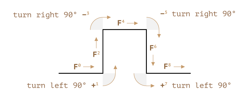
not very useful as it is, but we’ll now consider each symbol as a drawing instruction using the following rules:

• F draw forward
• + turn left 90°
• - turn right 90°

Let’s focus on iteration 1, F+F-F-F+F, and decompose each step:

You can use the following code to generate an array of segments from the l-system result (for the sake of simplicity, I’ll use the victor library for 2D vector):

const { segments } = result.split('').reduce(({ angle, segments }, symbol) => {
if (symbol === '+') return { segments, angle: angle - Math.PI * .5 }
if (symbol === '-') return { segments, angle: angle + Math.PI * .5 }
return { angle, segments: [
...segments,
// we create the segment, rotate it by the current angle and add previous position
(new Victor(20, 0)).rotate(angle).add(segments[segments.length - 1]),
]}
}, { angle: 0, segments: [new Victor(0, height)] })

Assuming you’ve got a CanvasRenderingContext2D, you just have to iterate through the array of segments to let the magic happen:

“const ctx = canvas.getContext(‘2d’)
ctx.beginPath()
segments.forEach(({ x, y }, i) => ctx[${i === 0 ? 'move' : 'line'}To](x, y))
ctx.stroke()

Not bad, in approximately 30 loc, you’ve got a graphic generated by an algorithm, try to reproduce this in your favorite graphic editor (illustrator, photoshop, krita…), you’ll see it’s not that simple, you can find the corresponding pen here.

It’s quite easy to implement the Sierpinski triangle or the Dragon curve using this technique.

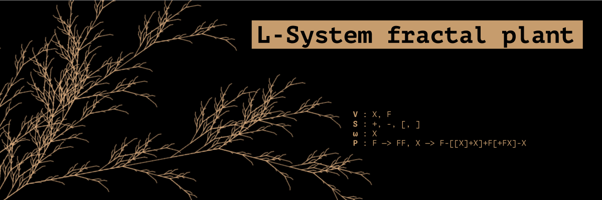
Second take: a fractal plant

For this one, we’ll add some constants and variables:

• variables V: X, F X is just a placeholder and won’t be interpreted during rendering phase
• constants S: +, -, [, ]
• axiom ω: X
• rules P: F → FF, X → F-[[X]+X]+F[+FX]-X

which will produces:

iteration 0 : X
iteration 1 : F-[[X]+X]+F[+FX]-X
iteration 2 : FF-[[F-[[X]+X]+F[+FX]-X]+F-[[X]+X]+F[+FX]-X]+FF[+FFF-[[X]+X]+F[+FX]-X]-F-[[X]+X]+F[+FX]-X

We can keep the same generation code, but we have to change the configuration accordingly:

const result = lSystem({
axiom: 'X',
rules: {
F: 'FF',
X: 'F-[[X]+X]+F[+FX]-X',
},
iterations: 6,
})

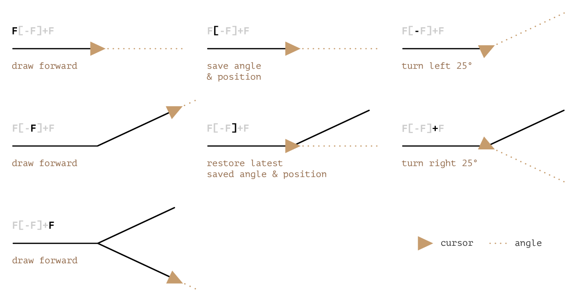
You probably noticed the addition of [ and ] constants:

• [ means save current position and angle
• ] restore latest saved position and angle

Which gives us a LIFO stack allowing to build non continuous lines, ideal for the branching required to model a plant. Let’s see how it works

You have to modify the segments generation code to integrate those new instructions and because it’s no more a continuous line, the segments are now composed of a start and end vectors:

const LENGTH = 6 // segment length
const ANGLE = 25 * Math.PI / 180 // angle used for rotations
const ORIGIN = new Victor(0, height * .95) // initial position

const instructions = {
'-': state => ({ ...state, angle: state.angle - ANGLE }), // turn left
'+': state => ({ ...state, angle: state.angle + ANGLE }), // turn right
'[': state => ({ // save position & angle
...state,
stack: [ ...state.stack, _.pick(state, ['position', 'angle']) ],
}),
']': ({ stack, ...state }) => { // restore latest saved position & angle
const last = stack.pop()
return { ...state, stack, ...last }
},
'F': state => { // draw
const end = new Victor(LENGTH, 0)
end.rotate(state.angle).add(state.position)

return {
...state,
position: end,
segments: [
...state.segments,
{ start: state.position, end },
],
}
},
}

const { segments } = result.split('').reduce(
// if the current symbol matches an instruction, use it, otherwise just return current state
(state, symbol) => (instructions[symbol] ? instructions[symbol](state) : state),
// initial state
{
angle: -30 * Math.PI / 180, // used to orient the tree
position: ORIGIN,
stack: [],
segments: [],
}
)

An update is also needed on the canvas code:

const ctx = canvas.getContext('2d')
ctx.beginPath()
segments.forEach(({ start, end }) => {
ctx.moveTo(start.x, start.y)
ctx.lineTo(end.x, end.y)
})
ctx.stroke()

That’s it, we now have the required code to build an almost natural organism resulting in the image at the top of this section, you can find the corresponding pen here.

There are infinite possible variations playing with rules/angle/length, if you google for L-Systems, you’ll probably find some pre-defined ones.

Conclusion

Thank you Aristid! I don’t think he anticipated the fame to come while conducting his research.

Apart from providing an easy way to get started with creative coding, it illustrates quite well that complex problems can (and should) be tackled with simple elegant solutions. Next time you’re having headaches implementing a complex recursive algorithm, don’t forget the rewrite trick.

If you liked L-Systems or you’re just interested in creative coding, you should have a look at the Paul Bourke website,  it’s a true goldmine!

I’m willing to write an article on how to add some randomness inside your L-System (using stochastic grammars), so stay in touch!

References

• https://en.wikipedia.org/wiki/L-system
• http://algorithmicbotany.org/papers/abop/abop-ch1.pdf
• http://www.modularbrains.net/support/SteliosManousakis-Musical_L-systems.pdf
• http://paulbourke.net/fractals/